This article explains how correlated or bunched requests can impact capacity planning results. An especially important example is the impact of highly correlated Internet traffic on sizing buffers in IP routers and HTTP servers.
1. Theorem of Threes
You’ve heard the expression, ‘’Things always happen in Threes!’’ For example: ‘’Three strikes, you’re out!’’ ‘’Three’s a crowd,’’ and ‘’Third time lucky!’’ Some people have even suggested that a ternary (base-three arithmetic) digital computer may have certain advantages.
If you’re a commuter waiting for a train or a bus, you may have heard some passengers ask rhetorically, ‘’Why Do Buses Always Come in Threes?’’ [ Eastaway & Wyndham 1998]. If you’re a commuter who drives a car on a congested freeway, then you’re also familiar with the situation in which your lane suddenly stops dead while the lane next to you continues to move. You decide to suffer the hassle of changing into the moving lane only to find that it now comes to a stand-still while your previous lane begins to move!
Whether or not things come in threes, the one thing that all these examples have in common is that they involve some kind of bunching phenomenon. Bunching of buses, cars, trains or events. This bunching can be explained in terms of some rather unintuitive effects associated with the theory of queueing. Queueing theory sits behind tools like TeamQuest Model and Pretty Damn Quick which are used to analyze the performance and capacity of computer systems and networks. It has also been demonstrated over the last decade that Internet packets can become entraned in much the same way as cars bunching together on the freeway--with one small difference. Instead of the cars bunching for just a few minutes to an hour, it’s as if they were to remain bunched for upwards of 10,000 hours!
So, it is well to understand some of these less expected queueing effects from the standpoint of computer system capacity planning and that’s precisely what we shall do in this online article.
2. Bus Paradox
There is an old conundrum in queueing theory that goes like this. A passenger arrives at a bus-stop at some arbitrary point in time. Buses arrive according to a Poisson process (i.e., completely randomly) at the bus-stop on average every 30 minutes. How long can a passenger expect to wait for the next bus?
There are two answers one can give to this question, both of which appear quite logical. The passenger must wait, on average:
- 15 minutes because she arrives at some instant which is the average of the time between buses.
- 30 minutes because Poisson arrivals are memoryless and thus the time until the next bus is independent of how long it has been since the last bus.
Therein lies the apparent paradox! The correct solution is explained in Section 3.1.
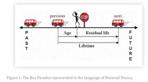
This is a particular example of a more general set of paradoxes that occur in a subject known as Renewal Theory which pertains to the breakdown of machines in a manufacturing plant due to ‘’aging’’. It turns out that we can also represent the Bus Paradox in terms of machine aging.
Referring to Figure [1], buses arrive from the right (i.e., the future) and depart to the left (i.e., the past). The interval of time between each buses is shown by the spacing between them. A some random time a prospective passenger arrives at the bus stop and waits for the next bus to arrive.
In the language of Renewal Theory, the interval between buses is called the ‘’Lifetime’’ because it would normally correspond to the time between the installation and breakdown of a machine. The time when the prospective passenger arrives at the bus stop corresponds to the time when a machine is inspected for maintenance. Not too surprisingly, this interval is called the ‘’Age’’ of the machine i.e., how old it is since it was installed. The period of time remaining until the machine actually breaks down is called the ‘’Residual Life’’ and that’s precisely the quantity we are interested in because it corresponds to the amount of time our passenger must wait.
More formally, the average or mean Residual Life [Kleinrock 1975] is given by:

where m1 is the mean Lifetime and σ2 is the variance about that mean. The important thing to note about equation 1 is that it not only involves the mean but also the variance of the Lifetime. In other words, averages on their own are not sufficient to determine the Residual Life.
Now, this is all very fascinating but how can we make sense of equation 1 in terms that are more familiar to a performance analyst? For that, we turn to queueing theory.
3. Queuing Models
Instead of considering the arrival of multiple buses at a bus-stop, we could equally think of there being just a single bus which is in a service loop for some average period of time (the Service Time) and passengers form a queue while waiting for the bus to return.
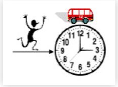
A rendition of this scenario is shown in Figure 2. The clock can be thought of as the ‘’server’’ with the single bus taking some average amount of time to complete the loop (around the clock). Passengers form a queue behind the clock. Since they will all embark together4 once the bus arrives, their individual waiting times are identical and therefore not of interest. What is of interest to them, however, is the average time they must all wait for the bus to return from its current service cycle i.e., Residual Service Time [Lazowska 1975, p.265].
Using the times mentioned in the previous section, let’s try to apply our queueing model to the Bus Paradox.
3.1 Random Buses: M/M/1
In queueing theory parlance, a single-server queue where both arrivals and service periods are random, is known as an M/M/1 queue. The ‘’M’’ can be thought of as standing for ‘’memoryless’’. The average waiting time is determined by the service time for each passenger (here assumed to be the same once they’re on the bus) multiplied by the number of passengers queued up at the bus-stop.

where Q is the average length of the waiting line. The mean queue-length in an M/M/1 queue is given by

where ρ is the fraction of time for which the server is busy. The average waiting time from equation 2 is thus,

To explain the Bus Paradox in Section 2, we assume that the average service period is S = 30 minutes and Q = 1 because all the passengers will embark together. Thus, the time a passenger can expect to wait is 30 minutes which is identical to a mean service period. That’s strange. It says that a passenger can expect to wait a complete service cycle no matter when they arrive at the bus stop!(?) A rather unintuitive result.
It’s unintuitive because we are, assuming that the bus service periods are completely randomized or totally uncorrelated in time. In reality they’re not, as was alluded to in our opening remarks. They may or may not come in threes, but they certainly are not uncorrelated. Next, let’s see what happens if we take correlations into account.
3.2 Correlated Buses: M/G/1
For M/M/1, the service periods are entirely uncorrelated. A more general kind of queueing model which allows for the presence of correlations in the service periods is called an M/G/1 queue. The ‘’G’’ stands for ‘’Generalized’’ as opposed to memoryless. The average waiting time is given by the famous Pollaczek-Khintchine [Gunther 2000] formula:

with cs2 = σ2 s2 the Squared Coefficient of Variation of the bus service time. The first factor looks the same as that for the M/M/1 queue in equation 2 but the second factor is new. It involves S and cs2 but not ρ. For this reason it is known as the Residual Service Time [Lazowska 1975, p.265]:

Notice how the residual Service time in equation 6 has the same form as the residual Life time in equation 1. The residual service time in our queueing model is the logical equivalent of the residual lifetime for machine breakdowns.
3.3 Deterministic Buses: M/D/1
From this M/G/1 queueing model of the Bus Paradox we see that the residual service time for the bus is very much affected by the value of cs2.
1. If the bus service periods are completely random, cs2 = 1 and Sresidual = S. This follows from the fact that completely random interarrival periods belong to the Exponential probability distribution whose variance is the square of its mean.
2. If the bus service periods are highly correlated, cs2 > 1 and Sresidual > S. A large Coefficient of Variation implies a large amount of variance. Large variance occurs when things get bunched up. If buses tend to arrive at the bus stop more or less together in bunches (of
three?) for a while then there must be long periods in the future where no buses arrive at all.
If the bus service periods were all equal (i.e., zero variance) then = 0 and Sresidual = ½S. In that case, there is no bunching at all. It corresponds to buses arriving at the bus stop like cars (or buses) on a manufacturing assembly line.
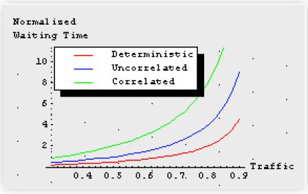
Figure 3 shows the differences in waiting times for each of these cases as a function of busyness of the buses.
4. Bunching Buses
So, do buses come in threes or not? We know from our queueing analysis that when you arrive at the bus stop, you are much more likely to have to wait for a period longer than the average service time because inter-bus arrivals tend to be more correlated than random and that tends to lengthen the residual service time. Put simply, you are more likely to chose a long interbus interval than a short one and correlations (M/G/1) will tend to make those intervals even longer than if they were purely random (M/M/1) periods.
We know that buses become correlated in the real world because groups of them leave their common depot together at the start of each day. They may get grouped on the roadways due to traffic congestion, and they get delayed at the bus stop itself. If there are a lot of passengers waiting first thing in the morning, they will tend to take a significant chunk of the service period to board the bus. This will tend to shorten the time until the next bus arrives.
[Eastaway & Wyndham 1998] go to great lengths to explain (qualitatively) that if buses do tend to bunch, they are more likely to come in pairs. I'll let you be the judge. Buses in Minneapolis have technology on board that keeps the inter-bus distance from bunching. Mexican bus drivers compete for the most passengers and adjust their speed to avoid bunching up at the bus stop (schedules are not a consideration, apparently).
5. Internet Bunching
We've seen how the residual service time of the bus is determined by cs2 ≥ o. What happens if i.e., cs2 → ∞ approaches some very large value?
It so happens that this case has already been measured on the Internet for more than 10 years. This ''infinite variance'' situation corresponds to large packet trains of data that persist for very long periods of time (on the time-scale of packets) from milliseconds to many minutes. This effect has been observed for all kinds of OSI application-level traffic: ethernet, HTTP, FTP, telnet, etc. Presumably, this phenomenon will become more ubiquitous as we invoke more and more multi-media streaming over the Internet.
Needless to say, this is potentially a very serious problem for capacity planning because buffers need to be sized to accommodate the mere possibility that large numbers of highly correlated packets may arrive at any time into routers or servers. A lot of passive resources may have to be assigned purely on a contingency basis. This can impact your budget for capital equipment!
A queueing model has been proposed which exhibits this infinite bunching effect:

where Q is the expected buffer size, and 0 < H < 1 is a special parameter called the ''Hurst Parameter'' 5 after Harold Hurst(1880-1978) who studied the highly unpredictable flooding 6 of the Nile river. Another form of bunching.
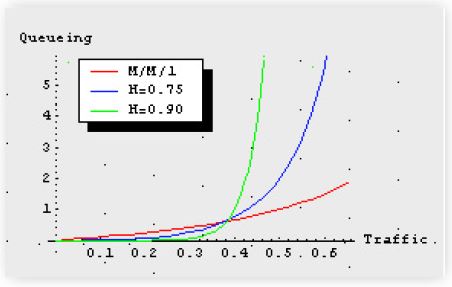
If H = 0.5, then equation 7 reduces to the queue length 3 for an M/M/1 queue. When large packet trains exist, H = 0.9 is a more typical value. The upshot is that buffers become floodedat relatively low traffic loads of the order of < 0.5 where an M/M/1 queue would only have an average queue length of 1. Figure 4 provides a graphical comparison of this astounding result. I go into more detail on this subject in my Guerrilla Capacity Planning class.
References
Allen, A., Probability, Statistics, and Queueing Theory with Computer Science Applications Academic Press, 1990.
Eastaway, R., and Wyndham, J., Why Do Buses Come in Threes? Wiley, 1998.
Probability Theory and It's Applications Vol.II Wiley, 1966.
Gunther, N. J., The Practical Performance Analyst, iUniverse.com Inc. 2000.
Kleinrock, L., Queueing Systems, Vol.I: Theory Wiley, 1975.
Quantitative System Performance: Computer System Analysis Using Queueing Network Models, Ed Lazowska, John Zahorjan, and Scott Graham, Prentice-Hall, 1984.
Mandelbrot, B. B., The Fractal Geometry of Nature Freeman, 1983.
Footnotes
1. Apparently, Mexican and Minneapolis buses never arrive in threes.
2. Humans have an innate predilection for making connections between otherwise random events. Our brains seem to be wired to ''see'' patterns or correlations even if they are not really there in any objective or repeatable sense. But why should we have a psychological preference for ''threes''? While composing this article the following idea occurred to me.
We need at least two ''similar'' events to define an interval of time: a ''start'' and an ''end''. Just like a sampling interval in performance measurement. Within that interval it is less difficult (subjectively) to find another ''similar'' event that supports our original choice of start and end events. Feeling validated, we stop ''looking'' for other correlations (no one talks about things happening in ''fours'' or ''tens'') and instead we turn our (short) attention to new things. If a third event seems not to occur, we forget the original interval-defining events altogether. We don't treat it as data disproving the Threes Theorem rather, we feel that the role of threes has been reaffirmed. And as if that were not bad enough (from a scientific standpoint), the temporal ordering can get rearranged if it suits the psychological purpose.
For example, someone who believes in the Threes Theorem reads that a famous Hollywood actor died and later they learn that a well-known politician died. What is the ''similarity'' between them? It could be that they are both famous, or that they both died or that they both lived in the same town, or whatever. There's a lot of subjective ambiguity in selecting the interval-defining end-points. The sequence looks like: Actor followed by Politician. The believer would now be looking (in principal) for an intermediate event: Actor, X, Politician. Instead, they recall that their pet goldfish died after both the Hollywood actor and the politician died. The fish was not famous but it does have death in common with the two people. After the fact, death defines ''similarity'' and instead of the goldfish's death representing an inclusive ''similar'' event it becomes mentally redefined as the ''end'' event: Actor, Politician, Goldfish. In other words, the temporal order can be chosen subjectively to reinforce the bogus Threes Theorem.
3. In which case you'd probably be late for work. (by a year)
4. The bus is actually a multi-server.
5. Hurst studied the ratio of the range R = (Max - Min) of the Nile river height to the standard deviation s=√{σ}2 for a number of years τ. He found that
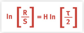
The Hurst parameter is the gradient of a straight line on a log-log plot. It corresponds to the fractal [ Mandelbrot] dimension in time rather than space, and it gives a measure of the amount of self-similar bunching.
6. A variant of: ''It never rains; it pours!''
Get started with a capacity management practice
Learn how to do capacity management and get to know the right tools for the job.
