This is an unexpected Part 3 to the discussion about the UNIX load average metric. Part 1 described what the kernel code does, while Part 2 explains how the load average actually computes the equivalent of something called an Exponential Moving Average (EMA), such as you find at BigCharts.com for doing stock market analysis. I say “unexpected” because
I thought I’d said everything there was to say about that topic. But recently someone asked me about where the weight factor Exp(5/60) comes from, and I realized I had somehow skipped over the details of that point. Here, I rectify that omission. As you’ll see, it’s a rather deep topic in itself. I hope you find it interesting and helpful.
Background
Just when you think you’ve said everything there is to say about a subject, up pops something that you’ve overlooked. Having already written three online articles and an addendum on the subject of how the load average is calculated in UNIX, I thought I had put the topic to bed.
However, at a recent CMG Conference (where I gave a presentation on this same topic) someone they did not understand how the weight factor exp(–5/60) arose in either the Linux code:
60 #define FSHIFT 11 /* nr of bits of precision */
61 #define FIXED_1 (1<<FSHIFT) /* 1.0 as fixed-point */
62 #define LOAD_FREQ (5*HZ) /* 5 sec intervals */
63 #define EXP_1 1884 /* 1/exp(5sec/1min) as fixed-point */
64 #define EXP_5 2014 /* 1/exp(5sec/5min) */
65 #define EXP_15 2037 /* 1/exp(5sec/15min) */
66
67 #define CALC_LOAD(load,exp,n) \
68 load *= exp: \
69 load += n*(FIXED_1-exp); \
70 load >>= FSHIFT;
or the equation:
L(t) = L(t-1) e-5/60 + n(t) (1 - e-5/60)
that appeared in my CMG paper as well as UNIX Load Average Part 2: Not Your Average Average, where L is the run-queue length or the system load in UNIX parlance.
On review, I believe my lunch-time interlocutor was quite right to point out that I did not do a very good job of explaining that particular feature. I also missed it in Chapter 4 of my new book, Analyzing Computer System Performance with Perl::PDQ. Therefore, I shall attempt to rectify the situation here by using the capabilities of Mathematica. The explanation turns out to be almost another paper in its own right!
BigCharts.com
In UNIX Load Average Part 2: Not Your Average Average, I pointed out that the expression:
L(t) = L(t-1) e-5/60 + n(t) (1 - e-5/60)
for calculating the UNIX load average is an exponential moving average (EMA). Exactly the same type of function is used to analyze financial data. In that case, the EMA gives more weight to the more recent price actions.
Here is a plot produced by BigCharts.com of the daily stock trading activity (black discontinuous curve) over the past year (2003–2004) for the New York Stock Exchange itself (in case you weren’t aware, NYSE is a publicly traded company–pause for thought in itself). The three colored curves are the 14 bar, 28 bar, and 42 bar exponential moving averages (EMA).
If you would like to make a chart like this for yourself, go to Interactive Charting, select Indicators, then Moving Averages, then EMA.
Mathematica 5.1 Configuration
The following packages are needed to enhance some of the Mathematica plotting functions.
Needs ["Graphics ` MultipleListPlot ` "]
Needs["Graphics ` Legend ` "]
Experimental Data
First, let's load in the data from my controlled experiments on my Linux platform.
paxRaw = Import["/Users/njg/TeamQuest/EMA Parameters/paxup2.cav"];
(Note the pathname nomenclature is for Mac OS X)
We then separate out the three curves corresponding to 1, 5, and 15 minute load averages,
paxLA1 = Flatten[paxRaw[[All, {1}]] ];
paxLA5 = Flatten[paxRaw[[All, {2}]] ];
paxLA16 = Flatten[paxRaw[[All, {3}]] ];
and plot them.
MultipleListPlot[Rest[paxLA1]. Rest[paxLA5], Rest[paxLA15],
PlotStyle → {Red, Green, Blue}, PlotJoined → True,
SymbolShape → None, PlotLabel → "Expermental Data",
AxesLabel → {"Sample", "LA1"}];
Unlike my CMG paper, note that the x-axis refers to the number of samples, not the number of seconds. Each sample was taken at 5-second intervals. Multiplying the sample number by 5 gives the elapsed time in seconds.
One-Minute Decay
For the sake of simplicity, we shall focus on the 1-minute decay data (red curve in the above Figure) which occurs somewhere after the 400-th sample point. Without loss of generality, our conclusions will apply equally well to the other curves.
paxDecayLA1 = Take[Rest[paxLA1], {420, 480}];
MultipleListPlot[paxDecayLA1, PlotStyle → {Red},
SymbolShape → {PlotSymbol[Triangle], None}
PlotLabel → "Decay Data",
AxesLabel → {"Sample", "LA1"}];
In the subsequent discussion it will prove useful to shift the origin of the x-axis (time steps) to the beginning of the decay sequence ,
Electric Circuit Analogy
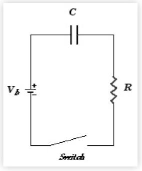
In UNIX Load Average Part I: How It Works, I remarked that the data from my controlled experiments reminded me of the charging and discharging of a capacitor in an RC circuit with resistor (R) and a capacitor (C). Let’s consider that analogy in a little more detail. Here is the schematic for a simple RC circuit:
Show[Import["/Users/njg/TeamQuest/EMA Parameters/RCFig02.gif"]]
The capacitor stores or releases a maximum amount of charge q = CV corresponding to the voltage drop (V) across the resistor, The relationship between these quantities is given by Ohm’s law V = IR where the electric current (I) corresponds to the change in the amount of charge over time i.e., I = Δq / Δt.
Ohm’s law can be rearranged to read R I = V which, after substituting the expressions for I and V in terms of the charge q, becomes:

This is a first-order differential equation describing the rate of change of the charge (i.e., the current) in the RC circuit. We can find the solution using Mathematica as follows (Mathematica prefers the notation y for q and x for t):
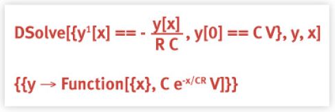
Restated in the notation of our RC circuit, the solution is:
q(t) = q(0) e-t/RC
As expected, the initial amount of charge in the capacitor is q(0) = CV, the maximum capacity (capacitance) described earlier. If we arbitrarily choose the values CV = 2, and RC = 12 in the discharge equation above, we see that it does indeed bear a striking resemblance to our load average data.
Plot[{e-t/12, 2e-t/12}, {t, 0, 60},
PlotLabel → "Capacitative Discharge",
AxesLabel → {"t", "q(t)"}, GridLines → {{12}, {0.368, 0.736}}];
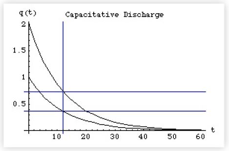
Another important characteristic is the time it takes the capacitor to reach 1/e of its original value. How much is that? Mathematica conveniently gives us the numerical value as:
N[e-1]
0.367879
or approximately 37% of q(0). Since q(0) = 2, the actual value is:
N[2e-1]
0.735759
According to our previous solution q(t) that point is reached when t = τ = RC. In the plot above it is indicated by the vertical straight line, by which we see that q(0) e-1 is reached at time τ = 12 units (no matter what the starting value q(0)). This time τ called the decay constant for the RC circuit and is fixed by the values of the resistor and capacitor. Once R and C are known, we know the characteristic decay curve of the circuit. But what has this circuit analysis possibly got to do with the load average?
Discrete Sampling
The preceding discussion assumed that we can specify the system at any point in continuous time (t). In the case of the load average, however, we have to sample the system at discrete points in time (the Linux kernel samples every 5 seconds. See UNIX Load Average: An Addendum). In other words, the differential equation that we wrote in the previous section has to be replaced by a difference equation.
Show[Import[*/Users/njg/TeamQuest/EMA Parameters/RCFig01.gif*]];
We used Ohm's law (V = IR) which corresponds to charging up the capacitor with a battery once, and letting it discharge across the resistor. The more general case allows for repeatedly charging up the capacitor with a generator or alternating voltage V(t). Then, the more general differential equation for an RC circuit has an extra term representing this alternating source of electrons:
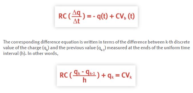
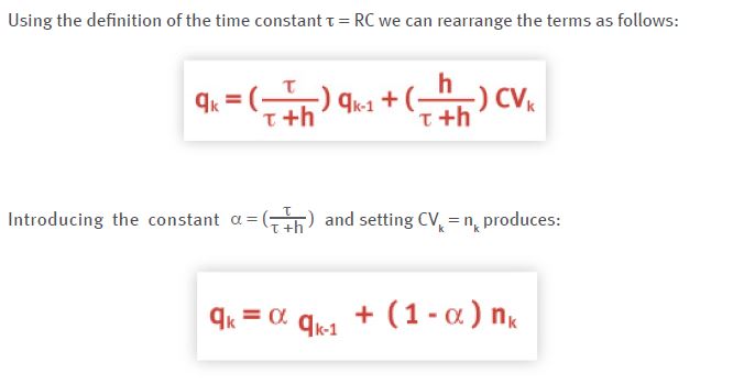
which has precisely the same form as the load average equation that I presented at CMG with α = exp(–5/60).
The RC time constant (τ) has been absorbed in the new constant (α), the sampled value of the electric charge (qk) at time step (k) corresponds to the sampled run-queue length, qk-1 is the previous sample of the run-queue, and the amount of charge remaining in the capacitor represents the number of active processes (nk).
Numerical Weights
We can think of the constant time period (τ) as being constructed of (k) samples or (k–1) sample
intervals each of length (h) i.e.,
τ = (k – 1) h
This expression corresponds to the time constant τ = RC in the electric circuit context.
Of course, in the context of the Linux load average there is no R or C to determine the value of τ. We do know, however, from the Linux kernel code that the sampling interval h = 5 seconds. If we tune the time constant (τ) to be the same as the reporting period (i.e., 1 minute or 60 seconds), then we require k – 1 =12 samples (or k = 13 divisions) during that period.
Using the above expression for (τ), the new time constant (α), introduced into the difference equation in the previous section, can now be expressed as:

from which it follows that

or the 1-minute difference equation.
Notice also that α = 12/13 and α = exp(-5/60) are numerically very close:
N[{12/13, e-5/60}]
{0.923077, 0.920044}
What this means is that after 12 steps, the constant α has been multiplied by itself 12 times and is very close to 1/e; the value of q(t) after one time-constant period (τ).

{13, 12/13, 0.382697, 0.367879, 0.367879}
So which weight is correct and why is α = exp(-5/60) used in the Linux code?
Linear Recursive Filter
Technically speaking, the difference equation
qk = α qk-1 + (1 – α) nk
for the sampled load average is known as a linear recursive filter because it acts like a lowpass filter that screens out any high frequency noise (spikes) in the measured signal. An RC circuit also acts as a low-pass filter (e.g., on a DSL-modified phone line).
The filter equation is linear because it does not contain any terms consisting of products or higher powers e.g., qk2. It is recursive because it does make use of values computed in the previous time step e.g., α qk-1.
Now, let's use this linear filter to model the decay portion of the Linux load average data. In that case, the difference equation simply becomes:
qk = α qk-1
which is computed as follows in Mathematica:

paxDecayEMA1 = Table[q = α q, {i, 0, 60}];
paxDecayEMA1 = Prepend[paxDecayEMA1, q0];
The last statement ensures that we have the initial value q0 at the beginning. The resulting list of values in paxDecayEMA1 is plotted as the red curve and the measured data is represented by the black triangles.
MultipleListPlot[paxDecayLA1, paxDecayEMA1,
PlotStyle → {Black, Red},
PlotJoined → {False, True},
SymbolShape → {PlotSymbol[Triangle], None}, GridLines → {{12}, {τ}},
PlotLable → "Comparative Decay",
AxesLabel → {"Sample", "LA1"}];
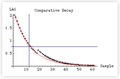
The agreement is excellent. Recall that the data (triangles) appear to lie above the theoretical curve in some regions because some Linux demons temporarily wake up to do some housekeeping. This means that the number of active processes being sampled is temporarily greater than the two CPU-intensive tasks under my control. Their long-run contribution, however, is damped out because they are short-lived processes (spikes). The net contribution over several samples therefore appears to be just slightly greater than the theoretical prediction.
In signal processing parlance the difference equation is called an infinite impulse response or IIR filter because the output response to an input signal continues indefinitely. My controlled Linux experiment was equivalent to measuring the IIR response to a step-function impulse i.e., I fired up two CPU-intensive background processes. The output would have remained at q(t) = 2 indefinitely but for the fact that I switched off the two background processes after 2100 seconds or 420 samples.
Load Lineage Revealed
To establish that these ideas are not new, I've included the following excerpt from The Instrumentation of Multics, by J.H. Saltzer (MIT) and J.W. Gintell (GE) published in August 1970 in the Communications of the ACM, Volume 13, Number 8. That's right, 35 years ago!
The section headings and the remarks are mine.
Recursive Equation
A variety of special purpose meters are therefore included as an integral part of the Multics multiprogramming scheduler and the page removal selection algorithm. Measures of paging activity include total processor time spent handling missing pages, number of missing pages, average running time between missing pages, and average length of the grace period from the time a page goes idle until its space is actually reused.
As a rough measure of response time for a time-sharing console user, an exponential average of the number of users in the highest priority scheduling queue is continuously maintained.
The exponential average is computed by a method borrowed from signal data processing [Blackman, R. B., and Tukey, J. W., The Measurement of Power Spectra. Dover, New York, 1958]. An integrator, I, initially zero, is updated periodically by the formula
I ← I × m + Nq, 0 < m < 1
where Nq is the measured length of the scheduling queue at the instant of update, and m is an exponential damping constant which determines the average distance into the past over which the average is being maintained.
Remark
This expression is identical to our difference equation:
qk = α qk-1 + (1 - α) nk
Weight Constant
In general, the sample which was taken k samples in the past, where
k = l / (l - m)
will have 1 / e times the effect of the current sample on the value of the integrator.
Remark
In our notation, this is equivalent to:
Average Queue Size
The average queue length is approximately
Nq = I / k
Remark
In our notation, this is equivalent to saying that the average queue length is given by the sum of all the samples divided by the number of samples (k).
CTSS and Multics
This averaging technique, which requires only a multiply and an add instruction slipped into a periodic path, is an economical way to maintain an average which does not "remember" conditions too far into the past.
If the recent average queue length is multiplied by the average run time in the first queue, an estimate is obtained of the expected response time of the moment. This estimate has been used on CTSS to dynamically control the number of users who may log into the system. In Multics, this estimate, as mentioned above, is also a guide with which to measure effectiveness of dynamic control of the size of the multiprogramming eligible set.
Conclusion
The answer to the original question (in the subtitle of this article) is more surprising than even I expected. Strictly speaking, the use of α = exp(–5/60) or exp(–1/12) in the Linux kernel macro as the damping factor in the 1-minute load average calculation is the result of either: (i) Linus getting mixed up while he was coding or (ii) Linus having mixed motives regarding accuracy (as explained here).
The correct numerical constant is α = 12/13, as discussed by the developers of Multics some 35 years ago. The Linux macro turns out to be a hybrid of the necessary discrete sampling of the real system load (the difference equation) and the time constant (τ) of the type seen in the continuous electrical RC-circuit model (the differential equation). Using the continuous damping
factor α = exp(–1/12) guarantees that after 12 samples the value of q(t) will be exactly α12 = 1/e of the original value.
That said, the degree of error between the two different expressions for the weighting factors is much less than 1% as Mathematica demonstrates. The discrete 1, 5, and 15 minute weights are respectively:
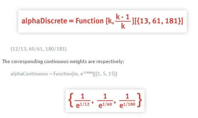
These results can now be tabulated:
TableForm[{alphaDiscrete, alphaContinuous, Clip[relativeError]},
TableDirections → {Row, Column",
TableHeadings →
{{StyleForm["Discrete", FontWeight → "Bold",
FontFamily → "Helvetica"],
StyleForm["Continuous", FontWeight → "Bold",
FontFamily → "Helvetica"],
StyleForm["% Error", FontWeight → "Bold",
FontFamily → "Helvetica"],
{StyleForm["LA01", FontWeight → "Bold",
FontFamily → "Helvetica"],
StyleForm["LA05", FontWeight → "Bold",
FontFamily → "Helvetica"],
StyleForm["LA15", FontWeight → "Bold",
FontFamily → "Helvetica"]}}] // N
Discrete Continuous % Error
LA01 0.9230769230769231` 0.9200444146293233` 0.32852174848998217`
LA05 0.9836065573770492` 0.9834714538216175` 0.01373552813555316`
LA15 0.994475138121547` 0.9944598480048967` 0.0015375061742747523`
Finally, we note that the magic numbers for the discrete sampling equation are:

which should be compared with the 1, 5, and 15 minute magic numbers used in the Linux kernel:
Function[m, Round[2048e-5/60m]][{1, 5, 15}]
{1884, 2014, 2037}
Only the 1-minute load average calculation is significantly affected.
Get started with a capacity management practice
Learn how to do capacity management and get to know the right tools for the job.
