This is the second in a two part-series where we explore the use of averages in performance analysis and capacity planning. Part 1 described some simple experiments that revealed how the load averages (the LA Triplets) are calculated in the UNIX kernel. In Part 2, I’ll compare the UNIX load averaging approach with other averaging methods as they apply to capacity planning and performance analysis.
1. Recap of Part 1
This is the second in a two part-series where I explore the use of averages in performance analysis and capacity planning. There are many manifestations of averages e.g., arithmetic average (the usual one), moving average (often used in financial planning), geometric average (used in the SPEC CPU benchmarks), harmonic average (not used enough), just to name a few.
In Part 1, I described some simple experiments that revealed how the load averages (the LA Triplets) are calculated in the UNIX® kernel (well, the Linux kernel anyway since that source code is available online). We discovered a C-macro called CALC_LOAD that does all the work. Taking the 1-minute average as the example, CALC_LOAD is identical to the mathematical expression:
load(t) = load(t - 1) e-5/60 + n(1 - e-5/60) (1)
which corresponds to an exponentially-damped moving average. It says that your current load is equal to the load you had last time (decayed by an exponential factor appropriate for 1-minute reporting) plus the number of currently active processes (weighted by a exponentially increasing factor appropriate for 1-minute reporting). The only difference between the 1-minute load average shown here and the 5- and 15-minute load averages is the value of the exponential factors; the magic numbers I discussed in Part 1.
Another point I made in Part 1 was that we, as performance analysts, would be better off if the LA Triplets were reported in the reverse order: 15, 5, 1, because that ordering concurs with usual convention that temporal order flows left to right. In this way it would be easier to read the LA Triplets as a trend (which was part of the original intent, I suspect).
Here, in Part 2, I’ll compare the UNIX load averaging approach with other averaging methods as they apply to capacity planning and performance analysis.
2. Exponential Smoothing
Exponential smoothing (also called filtering by electrical engineering types) is a general purpose way of prepping highly variable data before further analysis. Filters of this type are available in most data analysis tools such as: EXCEL, Mathematica, and Minitab. The smoothing equation is an iterative function that has the general form:

where X(t) is the input raw data, Y(t - 1) is the value due to the previous smoothing iteration and Y(t) is the new smoothed value. If it looks a little incestuous, it’s supposed to be.
2.1 Smooth Loads
Expressing the UNIX load average method (see equation (1)) in the same format produces:
load(t) = load(t-1) + EXP_R [ n(t) - load(t-1) ] (3)
Eqn.(3) is equivalent to (2) if we chose EXP_R = 1 - a. The constant a is called the smoothing constant and can range between 0.0 and 1.0 (in other words, you can think of it as a percentage). EXCEL uses the terminology damping factor for the quantity (1 - a).
The value of a determines the percentage by which the current smoothing iteration should for changes in the data that produced the previous smoothing iteration. Larger values of a yield a more rapid response to changes in the data but produce coarser rather than smoother resultant curves (less damped). Conversely, smaller values of a produce very smoother curves but take much longer to compensate for fluctuations in the data (more damped). So, what value of a should be used?
2.2 Critical Damping
EXCEL documentation suggests 0.20 to 0.30 are ``reasonable’’ values to choose for a. This is a patently misleading statement because it does not take into account how much variation in the data (e.g., error) you are prepared to tolerate.
From the analysis in Section 1 we can now see that EXP_R plays the role of a damping factor in the UNIX load average. The UNIX load average is therefore equivalent to an exponentiallydamped moving average. The more usual moving average (of the type often used by financial analysts) is just a simple arithmetic average with over some number of data points.
The following Table 1 shows the respective smoothing and damping factors that are based on the magic numbers described in Part 1.
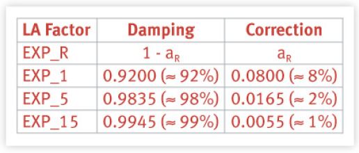
The value of a is calculated from 1 - exp(-5/60R) where R = 1, 5 or 15. From Table 1 we see that the bigger the correction for variation in the data (i.e., aR), the more responsive the result is to those variations and therefore we see less damping (1 - aR) in the output.
This is why the 1-minute reports respond more quickly to changes in load than do the 15-minute reports. Note also, that the largest correction for the UNIX load average is about 8% for the 1-minute report and is nowhere near the 20% or 30% suggested by EXCEL.
3. Other Averages
Next, we compare these time-dependent smoothed averages with some of the more familiar forms of averaging used in performance analysis and capacity planning.
3.1 Steady-State Averages
The most commonly used average used in capacity planning, benchmarking and other kinds of performance modeling, is the steady-state average.
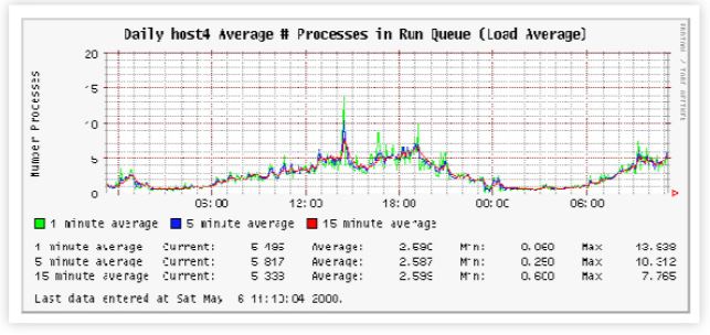
In terms of the UNIX load average, this would correspond to observing the reported loads over a sufficiently long time (T) much as shown in Fig. 1.
Note that sysadmins almost never use the load average metrics in this way. Part of the reason for that avoidance lies in the fact that the LA metrics are embedded inside other commands (which vary across UNIX platforms) and need to be extracted. TeamQuest IT Service Analyzer is an excellent example of the way in which such classic limitations in traditional UNIX performance tools have been partially circumvented.
3.2 Example Application
To determine the steady-state average for the above time series we would first need to break up the area under the plot into set of uniform columns of equal width.
- The width of each column corresponds to uniform time step Δt.
- The height of each column corresponds to Q(Δt) the instantaneous queue length.
- The area of each column is given by Q(Δt) * Δt (length * height).
- The total area under the curve is ΣQ(Δt) * Δt
The time-averaged queue length Q (the steady-state value) is then approximated by the fraction:

The longer the observation period, the more accurate the steady-state value.
Fig. 2 makes this idea more explicit. It shows a time period where six request become enqueued (the black curve representing approximate columns).
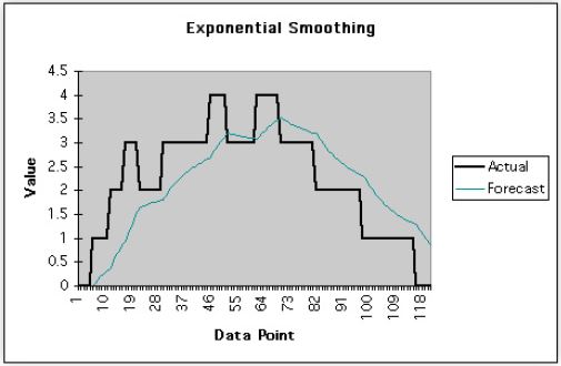
Superimposed over the top is the curve that corresponds to the 1-minute load average.
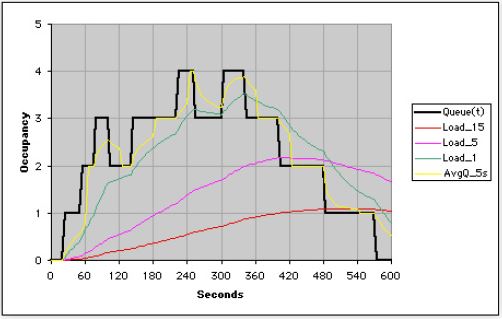
Fig. 3 shows all three load average metrics superimposed as well as the 5-second sample average.
3.3 Little’s Law
Consider the UNIX Timeshare scheduler.
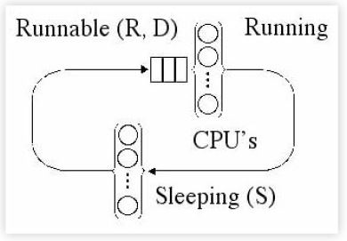
The schematic in Fig. 4 depicts the scheduler states according to the usual UNIX conventions:
- N: processes in the system
- R: running or runable processes
- D: uninterruptible processes
- S: processes in a sleep state
Applying steady-state averages of the type defined in Section 3.1 to other well-known performance metrics, such as:
- Z: average time spent in sleep state
- X: average process completion rate
- S: average execution quantum (in CPU ticks)
- W: total time spent in both running and runable state
allows us to express some very powerful relationships between them and Q (the steady-state queue length).
One such relationship is Little’s Law
Q = X W
which relates the average queue length (Q) to the average throughput (X) and the time (W):

In some sense, Q is the average of the load average.
These same kind of averages are used in performance analyzer tools like Pretty Damn Quick and TeamQuest Model.
Note, that such insightful relationships are virtually impossible to recognize without taking steady-state averages. Little’s law is a case in point. It had existed as a piece of performance folklore many years prior to 1961 when J. D. Little published his now famous proof of the relationship.
4. Summary
So, what have we learnt from all this? Those three little numbers tucked away innocently in certain UNIX commands are not so trivial after all. The first point is that load in this context refers to run-queue length (i.e., the sum of the number of processes waiting in the run-queue plus the number currently executing). Therefore, the number is absolute (not relative) and thus it can be unbounded; unlike utilization (AKA ``load’’ in queueing theory parlance).
Moreover, they have to be calculated in the kernel and therefore they must be calculated efficiently. Hence, the use of fixed-point arithmetic and that gives rise to those very strange looking constants in the kernel code. At the end of Part 1 I showed you that the magic number are really just exponential decay and rise constants expressed in fixed-point notation.
In Part 2 we found out that these constants are actually there to provide exponential smoothing of the raw instantaneous load values. More formally, the UNIX load average is an exponentially smoothed moving average function. In this way sudden changes can be damped so that they don’t contribute significantly to the longer term picture. Finally, we compared the exponentially damped average with the more common type of averages that appear as metrics in benchmarks and performance models.
On average, the UNIX load average metrics are certainly not your average average.
Get started with a capacity management practice
Learn how to do capacity management and get to know the right tools for the job.
