This paper shows how to apply some of the scalability concepts introduced in the previous paper to the performance analysis of real computer systems.
1. An Elephant Story
Did you hear the story about three blind men and the elephant?
- The first blind man touched the elephant’s leg and exclaimed, ‘’This animal is like a huge tree!’’
- The second blind man happened to hold onto the elephant’s tail and rejoined: ‘’No, this animal is like a snake!’’
- The third blind man protested: ‘’You’re both wrong! This animal is like a wall.’’ (He was touching the elephant’s flank.)
Each blind man thinks he is right and the others are wrong, even though all three of them are all touching the same elephant.
Consider now three performance engineers who are not blind (at least, not in the above sense). They are reviewing performance data collected from a computer system none of them has ever seen.
- [Engineer 1] ‘’Wow! This system scales linearly!’’
- [Engineer 2] ‘’No it doesn’t! It has a maximum throughput of mumble diddlysquats-persecond.’’
- [Engineer 3] ‘’No, you’re both wrong, the optimal load for this system is mumble users.’’
As you’ll soon see (pun intended), all three analysts are talking about different aspects of the same thing, just like the blind men and the elephant
2. Server Scalability
In my previous TeamQuest Online web column , I discussed multiprocessor and cluster scalability.
Recapping the main points briefly:
- Scalability is not a number (it’s a function)
- A surprisingly simple function was presented (the ‘’Super-Serial Model’’)
- This function is expressed very simply in terms of the processor configuration (p) and two measurable parameters ( and )
- The parameter is a measure of the level of contention in the system (e.g., waiting on a database lock)
- The parameter is a measure of the level of coherency in the system (e.g., cache-miss latency)
- The Super-Serial Model tells us that there can be a maximum in the possible capacity of the system
Here, once again, is the Super-Serial scaling equation (See also [Gunther 2000] eqn. (6-24), p. 189]):

where C(p) = [X(p)/ X(1)] is the normalized throughput represented as the ratio of the throughput X(p) with p processors relative to the throughput X(1) with just a single processor. If the parameter is zero (e.g., no cache-misses), then equation 1 simply reduces to Amdahl's law [Amdahl 1967], [Gelenbe 1989], [Gunther 2000]:

The parameter σ lies in the range: 0 ≤ σ ≤ 1, and represents the percentage of serial execution in the workload.

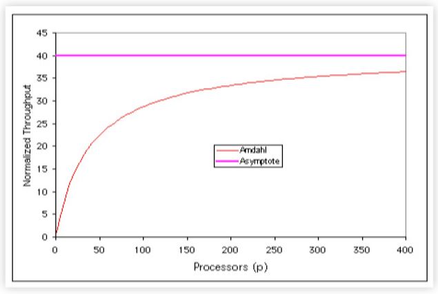
Unlike the Super-Serial model, Amdahl scaling does not have a maximum in its capacity function CA(p). Instead, it just has an asymptote at [1/(σ)] which is gradually approached as you add more physical processors into the system running the same workload. (See figure 1)
2.1 Example
Suppose the serial fraction is σ = 0.025 (i.e., it spends only 2.5% of the runtime in single-processor execution), then the multiprocessor will be executing in serial mode only 2.5% of the time (a rather benign fraction, right?). However, as you can see in figure 1, CA ∅ > 40 as p ∅. In other words, even if 400 physical processors could be electrically inserted into the backplane of the multiprocessor, it's effective throughput can never be better than 40 processors running at 100% busy.
In this sense, Amdahl's law represents a serious limitation or bound on the plausible system capacity and it's the subject of the remainder of this article.
2.2 Scalability is a Hot Topic!
As these current technologies attest: Peer2Peer, Apache, Windows 2000, Linux, the topic of scalability remains as hot today as it ever was.
An important point to note about equation 1 and equation 2, is that neither of these models (i.e., the equations) contains any reference to the kind of architecture used, or the interconnect technology, or the operating system or the application that is running. All those highly complex details are compacted into those innocent-looking σ and λ parameters. A very important result follows from this simplicity. These scalability models are universally applicable!
It also turns out that all of our scalability analysis holds equally well for both processor scaling (based on p physical processor) and process scaling (based on N user processes). Let's look at some public-domain benchmark data from the SPEC website to see how this works.
3. SPEC Benchmark
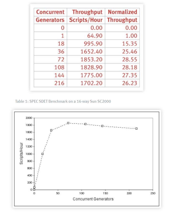
The SPEC benchmark that is most relevant for our scalability analysis is called SDET from the SDM (System Development Multitasking) Benchmark Suite which is currently part of the OSG (Open Systems Group) working group within the SPEC2 organization. The SDET3 workload simulates a group of UNIXTM software developers doing compiles, edits, as well as exercising other shell commands. These multiuser activities are emulated by concurrently running multiple copies of scripts containing the shell commands. The relevant performance metric is the throughput measured in scripts per hour. A very important distinguishing feature of the benchmark is that it does not rely on a single metric (as does CPU2000, for example). Rather, a graph showing the complete throughput characteristic must be reported. There are run-rules for SPEC SDM that indicate how this throughput data must be collected and presented.

The most significant features of this benchmark are:
- The throughput characteristic has a maximum
- The maximum throughput is 1853.20 scripts/hour
- It occurs at 72 generators (or emulated users)
- Beyond the peak, the throughput becomes retrograde
In a strange twist of fate, these measurements were done at Amdahl Corporation in Sunnyvale, California (the company founded by Gene Amdahl !).
Our three intrepid performance engineers (mentioned in the Introduction 1), might be heard to pronounce:
[Engineer 1] ''Wow! This system scales linearly up to 1652 scripts/hour!''
[Engineer 2] ''No it doesn't! It has a maximum throughput of 1853 scripts/hour.''
[Engineer 3] ''No, you're both wrong, the optimal load is 72 users.''
Obviously they are looking at the same data, but are they seeing everything that the benchmark data is trying to tell them? To get the most out of data like this, you need to have a performance model.
4. Performance Analysis
To construct a performance model it is usually necessary to have data on system resource consumption such as: process service times, disk busy, etc. In fact, the kind of data collected and reported by the TeamQuest View product. These same data can then be further processed automatically by the TeamQuest Model product.
Unfortunately, the SPEC SDET benchmark rules do not require the reporting of such system resource metrics, so we cannot proceed in that fashion. But all is not lost.
Clearly, the maximum measured throughput was 1853.20 scripts/hour. The SC2000 benchmark platform was configured and tuned to generate this maximum value (that's what the SPEC benchmarks are about). Moreover, part of this tuning is to make the system CPU-bound (not memory bound or I/O-bound). So, we can presume there was a dominant bottleneck throttling the throughput performance: the CPU in saturation.
4.1 Estimating the Service Demand (Dmax)
Using the relationship (See [Gunther 2000] eqn. (3-13), p. 108]):

where Xmax denotes the maximum system throughput and Dmax is the service demand (or service time) at the bottleneck resource (the CPU in this case). Turning this equation around (inverting) we get:

Since we know Xmax = 1853.20 scripts/hour from the data in figure 2, we can calculate Dmax = [1/ 1853.20] = 0.00054 hours (per script) or 0.00054 x 3600 = 1.94 seconds per script.
4.2 Estimating the Thinktime (Z)
We don't know the thinktime [Gunther 2000] parameter (Z) from the SPEC benchmark data, but we can estimate it. Using the relationship (See [Gunther 2000] eqn. (3-17), p. 109]):

We can simply read off X(1) = 64.90 (scripts per hour) from table 1, we have already calculated Dmax = 0.00054 hours , so we can just ''plug-and-chug'' to calculate Z in equation 6. The result is Z = 0.01487 hours.
4.3 Estimating the Optimal Load (N*)
A simple estimator of the optimal number of users [Gunther 2001] the system can support is given by:

where ( ∈*° ) means the floor function (or round down to the nearest whole number). Substituting the appropriate values from our performance model, we find N* = 28 (much lower than the measured saturation point of 72 generators).
If the average user load is maintained too far below this optimum (i.e., N << N*) the system capacity is under-utilized i.e., you're not using the resources for which you've already paid. Conversely, if the user load is maintained too much above this optimum (i.e., N >> N*) the system will become bottlenecked and response times will increase dramatically.
4.4 Simple Model
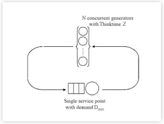
Now, we can construct a simple queueing model of this benchmark system using tools such as TeamQuest Model or PDQ (Pretty Damn Quick ©). The following figure 3 gives a schematic representation of the relationship between the benchmark generators (representing users) and the service point (representing resources).

To construct this simple model we need three parameters from the benchmark:
- The maximum number of users (N = 216 generators)
- The maximum service demand (Dmax = 0.00054 hours)
- The thinktime for each user (Z = 0.01487 hours)
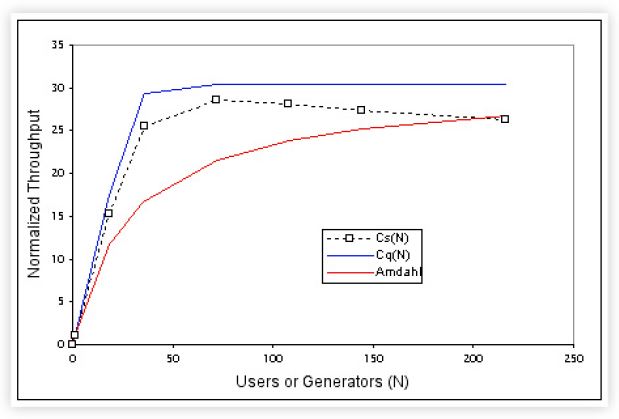
The normalized results of this analysis are shown in the following graph.

The queueing model (the blue curve) represents the best possible outcome one could expect from this benchmark platform. The measured data adheres fairly closely to the queueing model until it gets above CPU saturation, at which point the throughput falls somewhat below the simple theoretical expectations and throughput declines toward the Amdahl bound (in red).
4.5 Interpretation
This very simple queueing model of the SPEC SDET benchmark data reveals a tremendous amount of information about the performance of this ''elephant.'' Where one might have expected to build a simulation model of this otherwise complicated multiprocessor platform, we have actually arrived at a very close approximation to its benchmark performance characteristics using a queueing model with just a single service point. A real multiprocessor system has many service points e.g., memory-bus arbitration, spin-locks, i-node locks, just to name a few. Remarkably, we have subsumed all this detail into a single service point without too much loss of generality or accuracy. How did we get away with it!?
Aside: The key concept to recognize is the single service point corresponds precisely to the goal of making the benchmark workload CPU-bound (Recall the workload represents multiple UNIX software developers). It is a stress test. This also has the side effect of making the throughput characteristic (the blue curve in figure 4 rise almost linearly to the saturation plateau.
Real software developers would have significant thinktimes and a real multiprocessor system would have multiple service points. Those additional service points would tend to move the blue curve more towards the Amdahl bound. In other words, the ''real-world'' throughput characteristic would tend to have a much slower rise to the saturation plateau.
Our single service point model does not account for the data falling away from the saturation plateau toward the Amdahl bound (the red line in figure 4). It could and I'll more about that shortly.
5. Meaning of the Amdahl Bound
The worst case scenario is represented by Amdahl's law (the red curve) which now takes the form: because it is expressed in terms of the number of user processes instead of the number of physical processors as it was in equation 2. Note that the benchmark configuration was fixed at p = 16 processors. The throughtput was then measured (See figure 2) as a function of the number of emulated users (N) or concurrent workloads (in SPEC terminology).
Aside: It is possible to enhance our simple queueing model to include the retrograde throughput seen in the SDET benchmark data shown in figure 2. We have assumed that the service demand (Dmax) is constant (e.g., 1.94 seconds). This gives rise to the saturation plateau (blue line) in figure 4. If we relax that assumption and permit the service demand to increase (in some fashion), the queue would persist even longer and the throughput would begin to fall. One way to achieve this effect is through the use of a load-dependent server (See p. 99 ff. [Gunther 2000])
You may be wondering how I was able to produce the Amdahl bound without knowing the value of the σ parameter. I discovered that the σ parameter is related to the values of the service demand (D) and the thinktime (Z) in the following way:

such that:
- σ = 0 corresponds to the case D = 0 (i.e., all thinking)
- σ = 1 corresponds to the case Z = 0 (i.e., all waiting)
For the values of D and Z from the SPEC benchmark data, I found σ = 0.033 or 3.3%. But what does the Amdahl bound mean?
The queueing model assumes that the benchmark system is in steady-state at each configuration where measurements are taken. No doubt this is true. That means some users (i.e., benchmark workload generators) are being serviced while others are ''thinking'' (what to do next, presumably). The model also assumes that no user can have more than one outstanding request for service i.e., another request cannot be issued by the same user until the previous one has been serviced.
The Amdahl bound represents a worst-case scenario where all the users issue their requests simultaneously! Consequently, all N requests get piled up at the service center. Moreover, all the users have to wait until all the requests have been serviced and returned to their respective owners before any further ''thinking'' can be done. This is an all-or-nothing situation; all users have requests are either waiting in the queue or thinking. Both these phases represent low throughput. The proportion of time spent all thinking to all waiting during some measurement period is what determines the actual value of σ in equation 9.
An analogous situation arises for the processor version of Amdahl's law for CA(p) in equation 2. The serial phase of the workload can be thought of in the following way. One processor makes a request for data. It could do it by contacting each of the other processors in turn until it gets the needed response. The remaining (p - 2) processors would continue to compute uninterrupted (i.e., the outstanding request and computation would be overlapped). But, as I have shown in Chapter 14 of my book [ Gunther 2000], that's not the dynamic described by Amdahl's law. Instead, a processor making a request for data BROADCASTS its request to all the other processors in the system. In order to process that request, all the other processors must stop computing and ''listen'' to (and process) the request. Once again, we have an all-or-nothing situation.
6. The Elephant’s Dimensions
So, how big is this elephant? Let's collect all the various estimates from our queueing model analysis.

The average thinktime is not a real number that can be identified with direct measurement (it's typically set to zero in the benchmark scripts) and should be treated here as a modeling parameter.
The first performance engineer 3 was essentially correct as far as he went. But it's the remainder of the throughput characteristic that tells the real story.
The second performance engineer 3 was not wrong but was perhaps guilty of being too literal. The benchmark system is being overdriven. This is a requirement of the ''bench-marketing'' goal which is to get the highest peak throughput number. That single peak number is more impressive to the casual observer when quoted out of context from the other measurements.
The third performance engineer 3 was too optimistic. The optimal load of 28 users is less than half that expected from the benchmark data (i.e., the peak at 72 users). As can be seen in figure 2, 72 generators has already driven the system into saturation and the engineer did not take this into account.
Needless to say, they are all talking about the same benchmarked ''elephant.'' The Amdahl bound (which the benchmark data does indeed approach) is the more likely throughput characteristic of a general multiprocessor application. There is usually a lot more worst-case serialization in applications than most people realize. Writing efficient multiprocessor applications is a very difficult task (See Appendix C, ''Guidelines for Making Multiprocessor Applications Symmetric'' in [ Gunther 2000] p. 387]). None of the three performance engineers mentioned this characteristic.
7. Summary
This article has attempted to show you how to apply some of the scalability concepts introduced in my previous web column: ''Commercial Clusters and Scalability'' to the performance analysis of real computer systems. Using the concepts applied here to SPEC benchmark data, you should now be able to estimate each of the above quantities for yourself using your own data.
As I suggest in my classes [Gunther 2001], if the SPEC SDM workload looks at all useful for the performance analysis and capacity planning you are doing in your shop, you might consider purchasing a copy of the SDM code for $1450 from SPEC.org and adjusting it to make your own benchmark. The workloads do not have to be pure SDM if you are not planning on reporting an official SPEC result (and most of you are not). Therefore, you could just as well use the SPEC scripts as a benchmark harness and insert a workload that is most meaningful for your shop.
If you're also running TeamQuest View, you could collect system performance data from the benchmark platform and use TeamQuest User Probes to collect the SPEC SDM application data and merge it into the same performance database. See my online article: ''How to Write Application Probes in TeamQuest Performance Software 7.1'' for more details about doing this.
Whatever you choose to do, I hope this article has encouraged you to consider using the above techniques to see performance information rather than simply look at performance data. There might be a performance elephant standing in your datacenter.
Get started with a capacity management practice
Learn how to do capacity management and get to know the right tools for the job.
